Le Moyne College CSC-151 Microsoft Excel 2003 Reference
When Microsoft Excel 2003 starts, the window looks like the following.
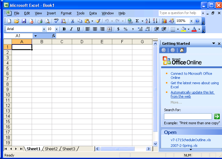
The graphical user interface (GUI) components that make up the normal view in Excel are as follows. These components are listed from the top of the window to the bottom.
| GUI Component | Description |
| title bar | The standard Microsoft Windows title bar that displays the name of the application and the name of the open spreadsheet file. |
| menu bar | Displays the Excel program menu. |
| standard toolbar | Contains buttons that are used to complete the most frequently used menu commands. |
| formatting toolbar | Contains buttons that are used to change the appearance or format of the spreadsheet. |
| formula bar | Contains the name box on the left (currently showing cell reference A1), the insert function button  , and a textbox that displays the contents of the active cell. , and a textbox that displays the contents of the active cell. |
| workbook window | Stores the information you enter in a grid of rows and columns. Rows are identified by number while columns are identified by letter. By default, three worksheet windows exist in a new spreadsheet file - Sheet1, Sheet2, and Sheet3 - as shown via the tabs found at the bottom of the worksheet window. |
| task pane | This is found to the right of the workbook window. It is used to display common tasks that are requested via the menu or a toolbar button. |
When Excel first starts, an empty spreadsheet file containing three worksheets and the "Getting Started" task pane is displayed. Cell A1 on Sheet1 is the active cell. The active cell is visually shown to you via the name box and the bold box drawn around the A1 cell.
Toolbars
As explained for Microsoft Word, a toolbar in Microsoft Excel may be achored either horizontally or vertically to the edge of the window, or it may float on top of the Excel window.
Task Pane
| The Getting Started task pane allows you to do any of the following: |
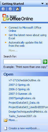 |
- Obtain the latest information about Microsoft Office and Excel via online resources.
|
- Open a recently used file.
|
- Open another file via the More... link.
|
|
Certain keyboard keys allow you to move the selected cell, called the active cell, to various locations within a worksheet.
| Keyboard shortcut | Action |
| <PageDown> | Move active cell down one full window. |
| <PageUp> | Move active cell up one full window. |
| <Alt> <PageDown> | Move active cell right one full window. |
| <Alt> <PageUp> | Move active cell left one full window. |
| <Home> | Move active cell to beginning of current row. |
| <Ctrl> <Home> | Move active cell to upper left corner of worksheet. |
| <Ctrl> <End> | Move active cell to lower right corner of worksheet. |
| <RightArrow> | Move active cell right by one column. |
| <LeftArrow> | Move active cell left by one column. |
| <UpArrow> | Move active cell up by one row. |
| <DownArrow> | Move active cell down by one row. |
| <End> <RightArrow> | Move active cell right to:- next used cell when active cell is currently empty.
- last contiguously used cell when active cell is currently not empty.
When no more cells are used to the right of the active cell, this keyboard shortcut moves the active cell to the right-most cell (always column IV) in the current row. |
| <End> <LeftArrow> | Move active cell left to:- next used cell when active cell is currently empty.
- last contiguously used cell when active cell is currently not empty.
When no more cells are used to the left of the active cell, this keyboard shortcut moves the active cell to the left-most cell (always column A) in the current row. |
| <End> <UpArrow> | Move active cell up to:- next used cell when active cell is currently empty.
- last contiguously used cell when active cell is currently not empty.
When no more cells are used above the active cell, this keyboard shortcut moves the active cell to the top-most cell (always row 1) in the current column. |
| <End> <DownArrow> | Move active cell down to:- next used cell when active cell is currently empty.
- last contiguously used cell when active cell is currently not empty.
When no more cells are used below the active cell, this keyboard shortcut moves the active cell to the bottom-most cell (always row 65536) in the current column. |
You may select a range of cells with either the keyboard or mouse, as follows.
| Keyboard | Mouse (assuming a right-handed mouse) | Description |
| <Shift> <RightArrow> | Click left-button on active cell and drag mouse pointer over cell to the right, release button when you've selected the appropriate cells. | Select a range of cells starting with the active cell and moving to the right. Number of selected cells is based on the number of times the <RightArrow> was pressed. |
| <Shift> <LeftArrow> | Click left-button on active cell and drag mouse pointer over cell to the left, release button when you've selected the appropriate cells. | Select a range of cells starting with the active cell and moving to the left. Number of selected cells is based on the number of times the <LeftArrow> was pressed. |
| <Shift> <UpArrow> | Click left-button on active cell and drag mouse pointer up over cells above the active cell, release button when you've selected the appropriate cells. | Select a range of cells starting with the active cell and moving up. Number of selected cells is based on the number of times the <UpArrow> was pressed. |
| <Shift> <DownArrow> | Click left-button on active cell and drag mouse pointer down over cells below the active cell, release button when you've selected the appropriate cells. | Select a range of cells starting with the active cell and moving down. Number of selected cells is based on the number of times the <DownArrow> was pressed. |
You may combine the above keyboard/mouse actions to select cells in multiple rows and/or columns. For example, if the active cell is C5 and you do a <Shift> <RightArrow>, then C5 and D5 are selected. If you then do a <Shift> <DownArrow>, the range of selected cells is now C5, D5, C6, and D6 (or C5:D6).
You may enter text or numbers into the active cell in any of the following ways:
- Simply begin typing.
- Double-click on the active cell then begin typing.
- Click on the textbox in the formula bar (immediately to the right of the insert function button
 ) then begin typing.
- Do an Edit, Paste (this assumes that you just previously did an Edit, Cut or Edit, Copy).
- Strike the <F2> key; the cursor is placed into the textbox in the formula bar, then begin typing.
To enter an Excel formula, you must begin by typing an equal sign (=). The equal sign is then followed by the Excel formula. The following are all valid examples of Excel formulas.
| Active Cell | Excel Formula | Description |
| A10 | =A1+A2+A3+A4+A5+A6+A7+A8+A9 | Computes sum of numeric values in cells A1 through A9 and displays result in A10. |
| A10 | =sum(A1,A2,A3,A4,A5,A6,A7,A8,A9 |
| A10 | =sum(A1:A9) |
| |
| G1 | =A1+B1+C1+D1+E1+F1 | Computes sum of numeric values in cells A1 through F1 and displays result in G1. |
| G1 | =sum(A1,B1,C1,D1,E1,F1) |
| G1 | =sum(A1:F1) |
| |
| C3 | =A1+B1+A2+B2 | Computes sum of numeric values in cells A1, B1, A2, and B2 and displays result in C3. |
| C3 | =sum(A1,B1,A2,B2) |
| C3 | =sum(A1:B2) |
You may change the text, numeric value, or formula in the active cell in any of the following ways:
| Method | Description |
| Simply begin typing | This will replace the current data in the active cell with whatever you enter. |
| Double-click on the active cell | The I-beam cursor appears in the cell; then do any of the following:
- Move the cursor using <LeftArrow> or <RightArrow> keys.
- Delete characters using <Backspace> or <Delete> keys.
- Enter data where appropriate.
When you are done modifying the cell value, you may hit <Enter> or click on another cell. |
| Click on the textbox in the formula bar | The I-beam cursor is placed into the textbox in the formula bar; then do any of the items listed for "Double-click on the active cell". |
| Strike the <F2> key | The I-beam cursor is placed into the textbox in the formula bar; then do any of the items listed for "Double-click on the active cell". |
Excel aligns data in a cell based on the type of data entered:
| Type of Data | Default alignment |
| Text | Left-aligned in cell. |
| Number | Right-aligned in cell. |
| Date (e.g., 5/31/2007) | Right-aligned in cell. |
| Time (e.g., 9:35) | Right-aligned in cell. |
You may change the default alignment of data using any of the alignment buttons found on the Formatting toolbar.
| Toolbar | Name | Description |
 | Align Left | Align the data along the left edge of the cell. |
 | Center | Center the data in the cell. |
 | Align Right | Align the data along the right edge of the cell. |
 | Merge and Center | Merge selected cells into one cell and center the data in this merged cell. |
To use the Merge and Center button, you must first select the cells that you want to merge into one cell. Generally, you should only select cells within one row or one column to merge and center at any one time.
You may also use the Format, Cells... menu to display the Format Cells dialog box. The Alignment tab in this dialog box allows you to align the active cell (or selected cells) horizontally and vertically. You may also change the orientation of the data displayed in the cell. Note that the Merge and Center button may be performed using this dialog box by selecting Center from the Horizontal text alignment dropdown list and checking the Merge Cells text control checkbox.
Note that when you use Merge and Center, the selected cells can no longer be referenced individually. For example, if you select cells C1, D1, and E1 then do Merge and Center, the resulting (larger) cell is known as C1, and cells D1 and E1 no longer exist! You can undo a Merge and Center by making the merged cell the active cell and clicking on the Merge and Center button.
You may change the width of a column using any of the following techniques.
| Technique | Procedure |
| Drag column boundary | - Position mouse over the column boundary in the column heading row (where the A, B, C, ... column headings are located).
The mouse pointer shape will change to 
- Click and drag the mouse pointer to the left or right depending on whether the column should be narrower or wider.
|
| Double-click on column boundary | - Position mouse over the column boundary in the column heading row (where the A, B, C, ... column headings are located).
The mouse pointer shape will change to 
- Double-click on the column boundary. The column width of the column to the left will be automatically adjusted to fit the widest data contained in this column.
|
| menu: Format, Column, Width... | - Select this item from the menu.
The Column Width dialog box is displayed.
- Enter a numeric value to adjust the width of the column that is currently selected.
|
| menu: Format, Column, AutoFit Selection | - Select this item from the menu.
- The column width of the selected columns will be automatically adjusted to fit the widest data contained in each column.
|
The height of a row may be similarly changed using a technique analogous to the above.
In Excel, the cut, copy, and paste features of Windows, which uses the Windows clipboard, acts differently from other software applications.
In the picture below, let's assume the user has done an Edit, Copy on cell A3, then moved the active cell to C3. The dashed box surrounding A3 will be animated in Excel (it will appear to be moving). This "moving" dashed box is a visual indication that a cut/copy operation has begun.
Note that if the user had instead done an Edit, Cut in cell A3, there would be no change to the picture above.
At this point, if the user does an Edit, Paste, the value 7500 will appear in the active cell C3. In addition the dashed box around A3 will still be "moving". Thus, we can do more Edit, Pastes to copy the 7500 value to other cells.
If we assume the user did an Edit, Paste in C3, D3, and E3, the diagram below shows the results.
Since the dashed box around A3 would still be "moving", we can continue to do Edit, Pastes to copy the 7500 value.
To cancel (terminate) the Edit, Copy, we can either strike the Escape key or start entering data into a cell. Either action will cause the dashed box around A3 to disappear. The removal of the moving dashed box around A3 visually signifies the end of the Edit, Copy operation.
Note that if the user had instead done an Edit, Cut in cell A3, the Edit, Paste operation on cell C3 would have resulted in the following picture.
As you can see, an Edit, Cut operation ends as soon as the Edit, Paste operation has occurred. Similarly, you can cancel an Edit, Cut by striking the Escape key or by starting to enter data into a cell.
Another way to copy data in a worksheet is to use the fill handle.
The fill handle is the small block square in the lower-right corner of the selected cells (active cells). In the picture above, A1 is the selected cell (active cell). The small black square where the gridline below row 1 and the gridline to the right of column A meet is the fill handle.
When you move the mouse pointer over the fill handle, the mouse pointer shape changes to a black plus sign 
To copy data, you would click and drag the fill handle when the mouse pointer shape is a black plus sign. Note that the fill handle does not use the Windows clipboard like Cut, Copy, and Paste.
To illustrate the difference between Copy/Paste and the fill handle, enter the text "dec" (without the quotes) in cell A1. Do an Edit, Copy in A1 then move to A2 and do an Edit, Paste, then move to A3 and do an Edit, Paste. The value "dec" was copied to these two cells.
Now enter the text "dec" (without the quotes) in cell B1. Use the fill handle to copy the B1 value to B2 and B3. As you can see, the B2 value is jan and the B3 value is feb. The fill handle interpreted "dec" as an abbreviation for December. So copying "dec" down the column resulted month abbreviations being created in sequence.
Feel free to enter a date or time value in a cell, then copy this value using the fill handle to observe the results of copying with the fill handle. Here are a few suggestions that you may want to try.
- Enter the date "02/26/2004" (without the quotes) in a cell and then copy it using the fill handle. Notice that the fill handle recognizes 2004 as a leap year so 02/29/2004 is listed as a date.
- Enter the date "02/26/2003" (without the quotes) in a cell and then copy it using the fill handle - no 02/29/2003 date!
- Enter "Nov 2000" (without the quotes) in a cell and then copy it using the fill handle.
- Enter "8:30 am" (without the quotes) in a cell and then copy it using the fill handle.
Microsoft Excel contains hundreds of predefined functions that perform computations.
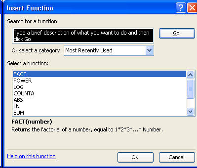
You gain access to all of these functions by clicking on the down arrow part of the AutoSum button  and selecting More Functions... from the dropdown list. The following dialog box is then displayed.
You can either enter a description of the function and click the Go button, or you can select a category from the dropdown list. The function categories are:
- Most Recently Used
- All
- Financial
- Date & Time
- Math & Trig
- Statistical
- Lookup & Reference
- Database
- Text
- Logical
- Information
- User Defined
- Engineering
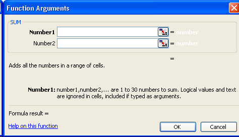
Once you select a function and click the OK button, the Function Arguments dialog box appears. The picture below shows the Function Arguments for the SUM function.
To use the Function Arguments dialog box, click on the Number1 textbox then use the mouse to select the cells. If you have a second range of cells that you want to include in the function, click on the Number2 textbox then use the mouse to select this second range of cells. And so on. When you are done, click the OK button and Excel will create the formula containing the function and cells you selected.
To help you select a range of cells using the mouse, you can reduce the size of the Function Arguments dialog box by click on one of the  buttons.
You may use the keyboard, mouse, or a combination to help you create an Excel formula.
Using a keyboard, you would simply start by typing in an equal sign (=) to denote a formula is in this cell. Then you would type in the formula you desire. To enter a cell reference, you would type the column identifier followed by the row identifer. You may use the following keys to represent various arithmetic operators.
| + | addition |
| - | subtraction |
| * | multiplication |
| / | division |
| ^ | exponentiation |
| % | percent |
Using a mouse, you would begin by clicking on the Insert Function button  found on the formula toolbar. You then use the mouse to click on a cell reference to include it in the formula. You would then use the keyboard to enter the appropriate arithmetic operator, and continue clicking on cell references and entering an appropriate arithmetic operator until you've entered the entire formula.
To insert a graphic (picture), select the Insert, Picture menu item. This displays a sub-menu containing the following choices:
| Insert, Picture sub-menu choices | Description |
| Clip Art... | Displays the Clip Art pane along the right edge of the Excel window.
Using this pane, you may search for clip art by typing in a keyword or phrase.
|
| From File... | Displays the Insert Picture dialog box.
Using this popup window, you browse through your computers storage devices looking for a picture (graphics) file.
You select the picture file and click the Insert button to insert the picture into your worksheet.
|
| From Scanner or Camera... | To use this menu item, you must have a scanner or camera connected to your computer, and this device must be turned on. |
| AutoShapes | Displays the AutoShapes toolbar (this may be a floating or fixed).
This toolbar contains buttons that allows your to select different shapes that you would select and draw on your worksheet. This feature is similar to the Drawing toolbar in Microsoft Word and Excel. |
| Word Art... | Displays the WordArt Gallery dialog box.
This feature is identical to the Word Art feature in Microsoft Word.
|
| Organization Chart | Inserts an organization chart template diagram and shows the Organization Chart toolbar.
You would then click on a chart's components to to modify its text value.
You add new components to the chart using the Insert Shape button found on the toolbar.
|
Once the graphic is inserted into your worksheet, you may format it by right-clicking on the graphic to bring up its shortcut menu. Towards the bottom of this menu you'll find Format Picture... (or Format WordArt..., Format AutoShape...) menu item that displays the corresponding dialog box.
- The Format Picture dialog box contains six tabs: Colors and Lines, Size, Picture, Protection, Properties, and Web.
- The Format WordArt dialog box contains five tabs: Colors and Lines, Size, Protection, Properties, and Web.
- The Format AutoShape dialog box contains one tab: Font.
One way to change the size of a graphic object is to click and drag its graphics handle (i.e., small circles found at the edge of the graphic object when you click on it).
A better way to change the size of a graphic object is through the Size tab. When using the Size tab, pay special attention to two options: lock aspect ratio and relative to original picture size. The lock aspect ratio ensures that the graphic object maintains the original ratio (proportion) of width to height. For example, if the original graphic has width of 2" and height of 3", any changes made to either the width or height will change the other value to maintain the 2 by 3 ratio.
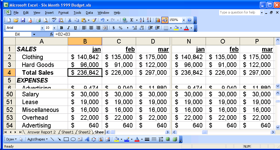
You can split an Excel window horizontally, vertically, or both. This allows you to view different sections of a worksheet simultaneously.
The picture below has been split both horizontally and vertically.
As you can see in this picture, we are viewing A1:D6 in the upper-left pane, N1:P6 in the upper-right pane, A50:D54 in lower-left pane, and N50:P54 in lower-right pane.
To split a worksheet horizontally, you click and drag the split box found immediately above the up arrow in the vertical scroll bar  .
.
To split a worksheet vertically, you click and drag the split box found immediately to the right of the right arrow in the horizontal scroll bar  .
.
You can freeze rows and/or columns at the top of a worksheet. This allows you to view row and/or column headings even though you have have scrolled far enough that the first few rows or columns should no longer be visible in the window.
The picture below shows row 1 and column A being frozen. Note the solid line between rows 1 and 2, and between columns A and B. The rows above and columns to the left of these solid lines have been frozen.
As you can see in this picture, we are viewing rows 1 and 234:243 and columns A and Q:V.
To do a freeze panes, make a particular cell the active cell and select Window, Freeze Panes from the menu. All rows above the active cell and all columns to the left of the active cell will be frozen.
To undo a freese panes, select Window, Unfreeze Panes from the menu.

 , and a textbox that displays the contents of the active cell.


 and selecting More Functions... from the dropdown list. The following dialog box is then displayed.
 buttons.
 .
. .
.