 or by selecting Insert, Chart... from the menu.
Microsoft Excel includes a chart making feature that is powerful and easy to use.
The easiest way to create a chart is to use the chart wizard, which you start by clicking on the Chart Wizard toolbar button  or by selecting Insert, Chart... from the menu.
While it is not required, it is a good idea to select the cells whose data you want to chart before you start the chart wizard.
The chart wizard contains four steps.
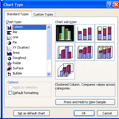
Step 1In this step you select the chart type and chart sub-type. The chart types are dispalyed in a listbox. The chart sub=types are displayed to you once you select a chart type. The picture shown shows the sub-types for the Column chart type. If you selected the cells prior to starting the wizard, you may click on the Press and Hold to View Sample button to see a preview of what your chart may look like. Detailed information about Excel chart types and sub-types can be found here. Click the Next button to advance to the next step. |

|
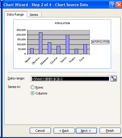
Step 2If you had selected your cells prior to starting the chart wizard, then you usually have nothing to do in this step. Note: the only thing you may want to adjust is whether the series should be by row or by column - the chart wizard determines this based on the chart type you've selected and the data found in the selected cells. If you have not selected your cells, now is the time to do it. Simply select the range of cells that contain the data you want to chart. When you've selected the cell range, the "Data range" textbox will show you the cell range. You may want to adjust whether the series is by row or column to see how this impacts your chart. Click the Next button to advance to the next step. |
|
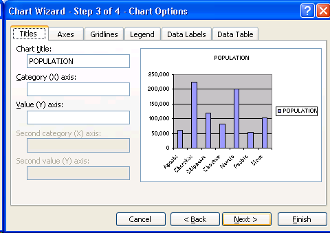
Step 3You have many options available to you in this step, per the six tabs found in this step.
Click the Next button to advance to the next step. |
|
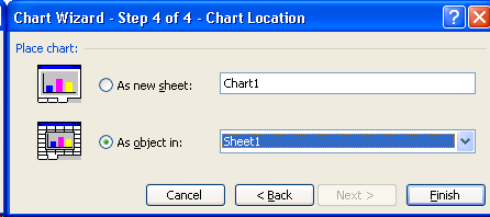
Step 4This last step allows you to indicate where the chart object should be placed. The default is to place the chart object inside the current worksheet ("as object in"). You may change the worksheet where the chart object is placed via the dropdown list. The other option is to create a new worksheet that will only contain the chart ("as new sheet"). In this case, you can use the default "Chart1" worksheet name or change this to another name. Click the Finish button to have Excel create the chart. |
|
Once the chart is created, you may move, size, format, and change the chart in many ways.
The entire chart object may be moved within the worksheet. Simply click on the chart object so that the graphic handles (i.e., small black squares) appear along the border of the object. Then click and drag the chart to the desired location. Note that when you create the chart "as new sheet" you do not have the ability to move the entire chart object.
You may move components found within the chart object by clicking and dragging the component within the chart. When you click on a chart component, the graphic handles should appear around only that component, then click and drag the component to the desired location within the chart object. The chart components that may be moved include the chart title, legend, and chart plot area (the chart itselt - which includes the axes and axes labels).
You may resize the entire chart object by clicking on the chart object so that the graphic handles (i.e., small black squares) appear along the border of the object. Then click and drag one of the graphic handles to make the chart larger or smaller depending on your needs.
You may resize a component found within the chart object by clicking on the component so that the grahpic handles appear only around the component. Then click and drag one of the graphic handles to make the chart component larger or smaller depending on your needs.
When you right click on the entire chart object or on a chart component, a shortcut (popup) menu appears. This menu indicates the actions you may take for the clicked object. The first item in this shortcut menu will allow you to format the clicked object. The chart components that may be formatted via its shortcut menu include the chart area, chart title, axis labels, legend, data series, plot area, and gridlines.
|
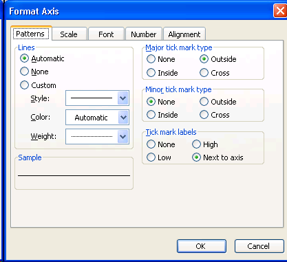
Of particular interest are some of the formatting options for the axis labels:
|
|
|
After the chart object is created, you are still allowed to change the chart type and sub-type. When you right-click on the entire chart object, the shortcut menu contains the item "Chart Type...". When you select this menu item the Chart Type dialog box appears, aloowing you to change the type and sub-type of the selectet chart object. |
|